Methodology
The time-of-week and temperature demand response model is trained using hourly energy usage intervals and predicts in hourly intervals, for use on short-term baselines.
The model is a time-of-week and temperature (TOWT) model, closely related to the original LBNL TOWT model.
Model Theory🔗
The model predicts hourly usage from three sources of variation:
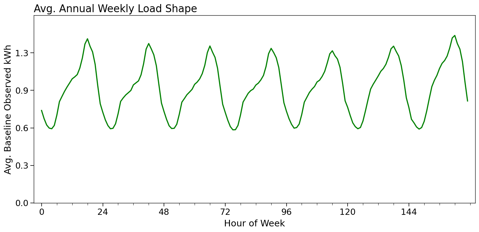
- Hour of week — the week is divided into 168 hourly intervals (starting Monday), capturing the recurring weekly load shape.
- Outdoor dry-bulb temperature — a binned temperature response.
- Occupancy state — whether the building is in a high-load (“occupied”) or low-load (“unoccupied”) mode for a given time of week.
A separate prediction is produced for each hour of the week, each carrying its inferred occupancy state — so, for example, Tuesday 7 pm, Friday 3 am, and Sunday 7 pm each get their own fitted behavior.
Occupancy🔗
Occupancy is not supplied as an input; the model infers it from the baseline data. Each of the 168 hours of the week is classified as either “occupied” (a high-load mode) or “unoccupied” (a low-load mode), and that classification is what lets the model treat, say, a weekday business afternoon differently from the same building overnight.
The classification is made by first fitting a simple weather-only regression of usage against heating and cooling effects, with fixed reference temperatures (cooling above 65 °F, heating below 50 °F). For every hour of the week, the model then looks at how the actual usage sits relative to that weather-only expectation. If more than 65% of the observations for an hour of the week fall above the weather-only prediction, that hour is marked occupied; otherwise it is marked unoccupied. The intuition is that hours where usage routinely exceeds the simple weather baseline correspond to periods of activity, while hours that sit at or below it correspond to a building’s idle state.
Temperature response🔗
Within each occupancy mode the response to outdoor temperature is captured with a binned (piecewise) scheme rather than a single slope, so the model can bend at the temperatures where heating and cooling behavior changes. Candidate bin edges at 30, 45, 55, 65, 75, and 90 °F divide the temperature range into segments. The bins are fit separately for occupied and unoccupied hours, allowing the two modes to respond to temperature in different ways. Where a candidate bin holds too few temperature readings to be estimated reliably, it is merged inward from the extremes, so sparsely populated cold or hot bins do not destabilize the fit.
Model components🔗
The fitted model is a sum of components, each capturing a distinct “bucket” of consumption:
- Temperature-independent (“always-on”) load across all hours of the week.
- Temperature-dependent usage during unoccupied hours.
- Additional temperature-independent usage during occupied hours.
- Additional temperature-dependent usage during occupied hours.
The occupancy classification, temperature binning, and the full hourly design matrix are specified in Sections 3.8–3.10 of the CalTRACK 2.1 Methods.
Single model🔗
Demand-response baselines are short, so this model fits a single TOWT model over the entire baseline period.
Additional details can be found in the CalTRACK 2.1 Methods and the Technical Appendix.