General Concepts
Why Predict Energy Usage?🔗
If you are new to the energy industry, you may be asking yourself what the use cases for predicting energy usage are. In truth, there are many use cases for predicting energy usage, and the ability to do so accurately has far-reaching consequences from the economics of a single household to the stability of the entire grid.
Common Use Cases Include:
- Forecasting load using weather forecasts to ensure adequate energy supply for the days, weeks, months, and years ahead.
- Determining the impact of interventions (an intentional change to a building to decrease energy usage) such as energy efficiency and demand response. This includes:
- Understanding the financial impact of installed interventions to accurately track ROI.
- Utilities measuring the impact of these interventions on the utility grid and effectively utilizing them as grid resources.
- Implementing “continuous commissioning” at buildings to track changes in energy usage and diagnose equipment issues.
- And many more…
In this documentation we’ll be focused on determining energy savings. After exploring this use case, you will have all the tools needed to apply OpenDSM for any use case desired.
Quantifying Energy Savings🔗
Within the realm of energy efficiency, there are many different ways to calculate energy savings. The fundamental problem in calculating energy savings is the production of a “counterfactual”. What would the energy usage have been in the absence of a specific intervention such as a new HVAC system? This is impossible to truly know, but several techniques are commonly used to accomplish this.
Deemed Savings / Engineering Estimates🔗
This method involves contrasting the current condition of the building with the future condition of the building. This may mean comparing an existing refrigeration system with a newly installed one that is twice as efficient, or perhaps estimating the impact of behavioral changes at a site that is adapting new working procedures.
The fundamental problem with this method is that it involves many assumptions. For example, what if the house that just installed the ultra-efficient refrigerator moves their old one into the garage? What if workers do not adapt the new working procedures as expected? Engineers and analysts can attempt to increase the accuracy of their calculations by spending more time tuning calculations to a specific site, but this increases overhead and takes time without any guarantee of increasing accuracy.
Contrasting Current Usage with Prior Usage🔗
This method involves simply comparing the current year’s usage vs. the previous year. Although this is quickly done and leverages real meter data, it disregards the difference in conditions between the two years - in particular, temperature - which can have a huge impact on the energy usage at a site.
Randomized Control Trial🔗
This method involves finding “nearly identical” sites that are not receiving interventions and comparing the energy usage to those receiving interventions. This side steps the temporal issue of different conditions in each year, but also introduces new challenges with finding “nearly identical” building to match with those receiving interventions. This can be difficult since no building is truly identical with its energy usage, but this can be compensated for with higher sample sizes and is best for residential programs.
Estimate Usage with a Model🔗
This method involves using a model to predict energy usage and then comparing it to the actual usage to determine savings. With EEmeter, this approach relies entirely on temperature and meter data to create a model that can be used to predict energy usage.
The pros of this method include:
- No need for ad-hoc assumptions - only actual meter data and temperature impact the model.
- Temperature data is used to accurately predict energy usage and contrast energy usage between different time periods.
- No need for finding “nearly identical” buildings.
- Method is suitable for most buildings.
In addition, when using EEmeter with default configuration, users can be assured of consistent methods to determine energy savings. This is a fundamentally important point when calculating energy savings - consistency. If five different people come up with five different answers, which one do you trust? If estimates are coming from parties that stand to benefit from higher savings estimates (such as energy service companies, engineers, contractors, etc), these numbers are even harder to trust. By using standardized methods, the savings calculations are deterministic and avoid dangerous assumptions.
Intervention Lifecycle🔗
When calculating savings from an intervention, it is important to define temporal periods as these impact how we train and use our model. For a typical efficiency intervention, we will define three periods:
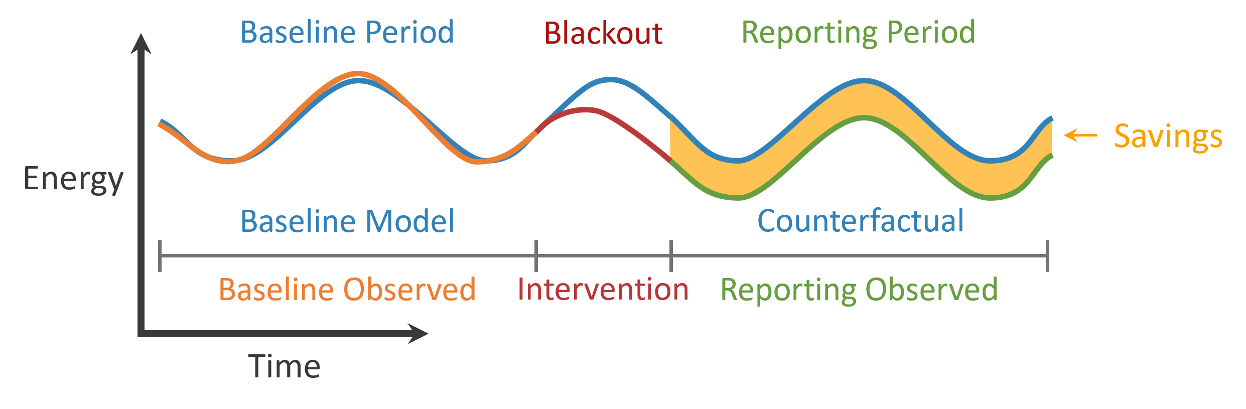
- Baseline Period: The period leading up to the intervention period that the model is trained on. For efficiency projects, this is 365 days. For demand response, the period may be shorter.
- Blackout Period: The period in which the intervention is being installed that should not be included in either baseline or reporting periods. During this period, energy usage is often erratic due to the installation process. For some interventions, the blackout period may be months, and for others there may be no blackout period (i.e. demand response).
- Reporting Period: The post-blackout period in which we can compare the model counterfactual to the observed energy usage to calculate savings. Reporting periods for efficiency projects typically last at least 365 days but may go far beyond this. For demand response, the reporting period is typically just the event day.
Error Metrics🔗
There are many possible error metrics that can be used to assess model performance. Within OpenDSM, three are commonly used: root mean squared error RMSE, mean absolute error MAE, and mean bias error MBE. Each metrics has its own set of pros and cons, and the choice of which should be used is dependent on the question being asked.
For model acceptance, OpenDSM uses RMSE. However, we cannot use RMSE without normalizing it because we must use generalized cutoff criteria. RMSE’s magnitude depends upon the baseline data from which the model is fit from. How to normalize the RMSE to make it reflect general model fit performance is not a simple matter though.
CVRMSE🔗
The coefficient of variation of the root mean squared error (CVRMSE) is one way to normalize a model’s error.
CVRMSE normalizes RMSE by the mean of the observed data over a given period of time, often the baseline for the purposes of model fit sufficiency. Another way to think about CVRMSE is the error as a percentage of average usage. CVRMSE fails as a useful metric when the mean usage is near zero or negative. Unfortunately, this is a common occurance with behind-the-meter generation such as solar PV systems.
PNRMSE🔗
Percentile normalized RMSE (PNRMSE) is a more recent measure of performance. PNRMSE normalizes by the IQR of the observed data over a given period of time.
Because PNRMSE normalizes by IQR, the denominator will always be positive. It will also stay at a reasonable magnitude for all meters with variation in their usage. It can be thought of as how large the error is relative to the variance of the observed data. There is still the possibility that a meter which has very little variation could still fail the PNRMSE threshold requirement for model sufficiency; this is why we use CVRMSE and PNRMSE together.
CVRMSE and PNRMSE Relationship🔗
PNRMSE sufficiency criteria have been derived from PNRMSE’s relationship to CVRMSE. 1000 meters were fit and their normalized erro metrics plotted against each other resulting in the following plot.
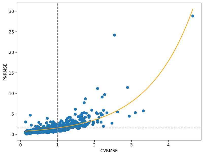
From this fit, it was determined that at a CVRMSE of 1.0, PNRMSE is 1.6, and at a CVRMSE of 1.4, PNRMSE is about 2.2.
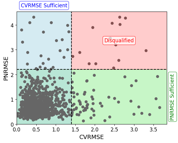
Combined Disqualification🔗
All models use a combination of CVRMSE and PNRMSE to disqualify models. This is done permissively. A model need only be qualified under one of the model sufficiency criteria. To visualize this, the following figure was generated assuming the hourly model thresholds.