Methodology
The hourly model is trained using hourly energy usage intervals and predicts in hourly intervals.
The hourly model has two, closely related variations: a non-solar and a solar model. The only difference between the two is that the solar model requires an additional solar irradiance input. For the purposes of this page, we will describe the solar model, but explanations are the same for the non-solar model except for the solar section.
Model Theory🔗
Model Algorithm🔗
The hourly model is built using an elastic net regression framework. During the development of the hourly model many algorithms and methodologies were considered including neural nets; however, elastic net regression proved to be the perfect blend of accurate and efficient.
The elastic net regression technique uses a linear regression model with regularization. Regularization enhances predictive capabilities by performing feature selection to limit unnecessary model complexity while maximizing model accuracy. Elastic net regression is itself the combination of lasso regression and ridge regression.
Lasso regression penalizes the absolute magnitude of model coefficients which has the effect of pushing those coefficients towards zero unless the balanced by an increase in model error in the form of sum of squares error. By pushing coefficients to zero when they do not help the model, the lasso component acts as the feature selection component.
Ridge regression penalizes the square of the model coefficients which has the effect of more harshly penalizing large coefficients thereby pulling the coefficients closer together in magnitude. This is one approach to handling multicollinearity as correlated variables will end up having similar coefficients.
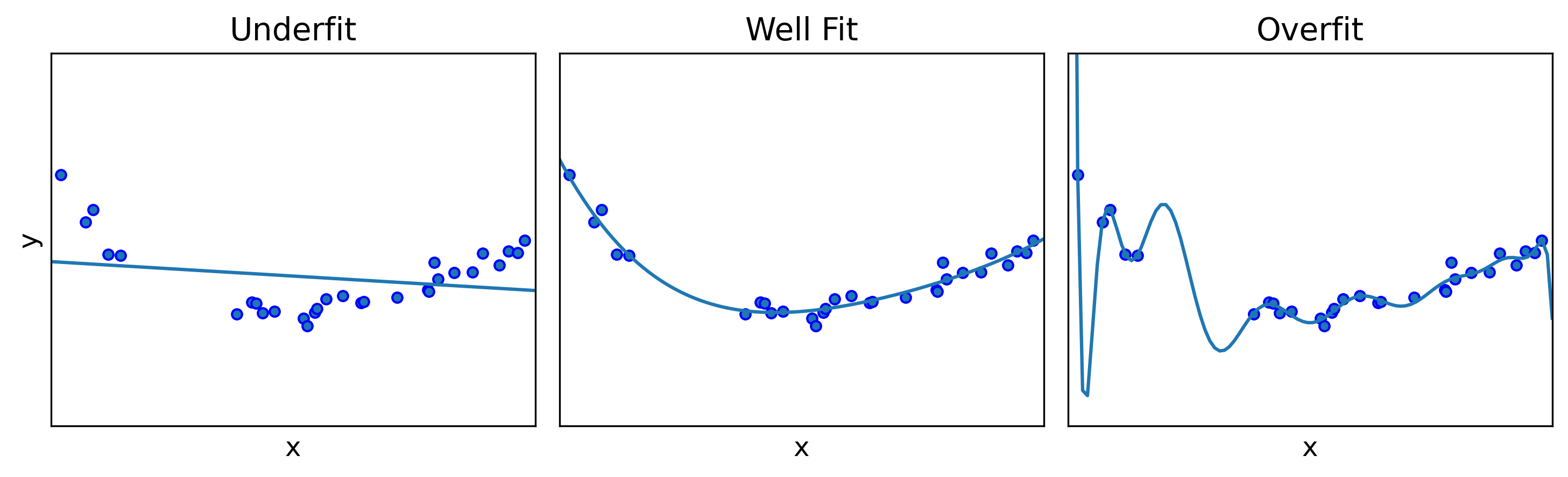
The hourly model relies heavily on feature selection to avoid overfitting with the goal of making a well-fit model. To prevent underfitting, we utilize Model Inputs that are correlated with usage.
Basic Fit/Predict Structure🔗
The input structure to the elastic net framework has been set up such that each hour of usage is informed by all 24 hours of the day. This inherently considers leading and lagging effects of all variables but most importantly temperature. This means that the model innately accounts for phenomena such as thermal lag and precooling if they are regularly part of a building’s usage behavior.
Model Inputs🔗
Correlation-based Imputation🔗
Inputs into the elastic net framework are required to be complete with no missing values. This is unrealistic for inputs into the hourly model so a correlation-based imputation methodology was developed to impute missing values for standard inputs. Autocorrelation is performed on each input and using the largest peaks (most correlated leads/lags) missing values are imputed using the most correlated values around them in time. Additional details can be found in the References.
Temperature🔗
Building energy consumption generally has a strong response to temperature, which varies considerably in different geographic regimes with different heating and/or cooling needs. For this reason, hourly temperature is a required input. To further clarify, hourly temperatures are the mean hourly outdoor dry-bulb temperature as measured at the nearest weather station within the same climate zone. Getting this information is handled in EEweather.
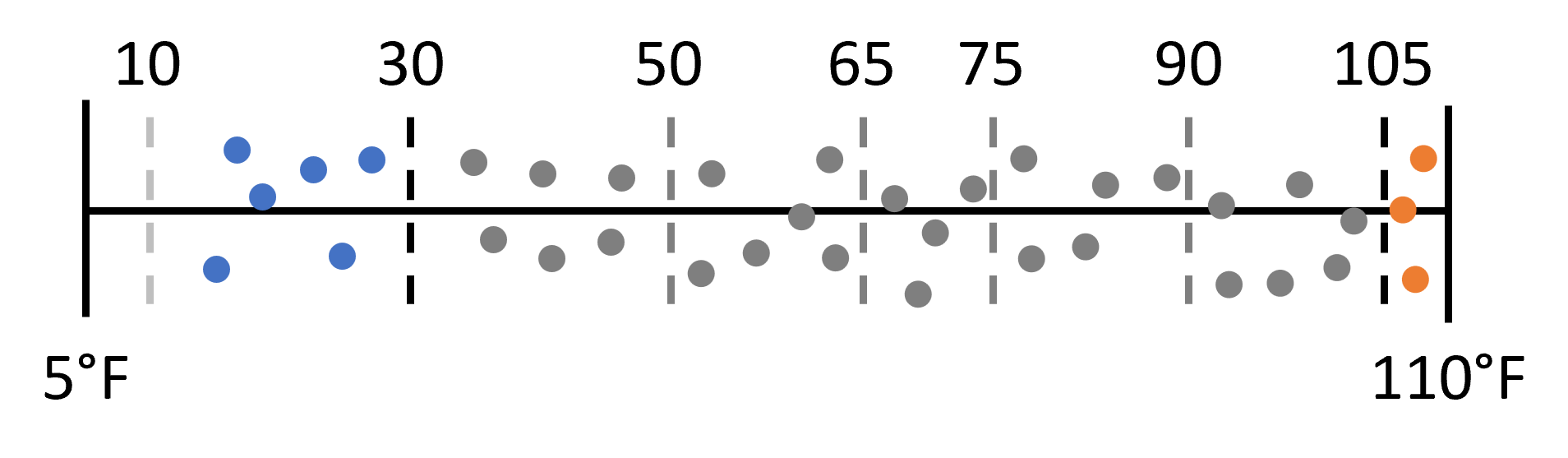
Usage can vary significantly and discontinuously as temperature changes. To model this behavior, the hourly model utilizes fixed temperature bins. Within each temperature bin, temperatures are given unique slopes and intercepts. This means that each temperature bin can respond linearly to the usage within its bin edges. The exact bin edges are shown in the figure below.
At very low and high temperatures, a building’s energy usage can start changing dramatically even within a temperature bin. This can happen for a number of reasons but HVAC is a primary driver. For example, at high temperatures an air conditioner can be in normal operation, be under increased load as inhabitants decrease the temperature, or be at maximum capacity. Each of these scenarios results in a different energy usage profile. Our model accounts for these swift changes by giving the lowest and highest populated temperature bins an additional non-linear components.
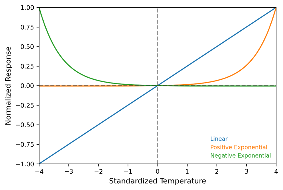
By adding the linear temperature response with the positive and negative exponentials, each fit with their own unique coefficients, it’s not hard to imagine the complexity that this structure could model.
Temporal Features🔗
Due to people’s behavior (among other drivers), time-of-day, day-of-week, and month can completely change how a building uses energy. The hourly model creates one hot vectors using day-of-week and month. Time-of-day need not be considered because of the 24-hour fit/predict structure. Creating one hot vectors for all combinations of day-of-week and month would undoubtedly create an overfit model in some circumstances, so the hourly model has a preprocessing routine to cluster the median daily usage profiles of all 365 days by day-of-week and month. Full details of this methodology can be found in the References. This procedure allows for the algorithm to automatically combine days in which energy consumption is similar and to separate those that are not.
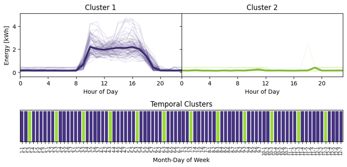
In this example, the building has a clear difference in energy consumption depending on if the day of week is Wednesday or any other day of the week. This is likely a commercial building that shuts down on Wednesdays.
Temperature Bin - Temporal Cluster - Temperature Interactions🔗
Temperature bins and temporal clusters can interact in unexpected ways. An office building, for example, might decrease their AC set point during off-hours when the temperature is high. The hourly model accounts for this by using the interaction between temperature, temperature bins, and temporal clusters. This means that the model has several different temperature reponse variables: global temperature response and a temperature response for all temporal clusters. The model calculates the combination of the global temperature response with the temporal cluster temperature responses.
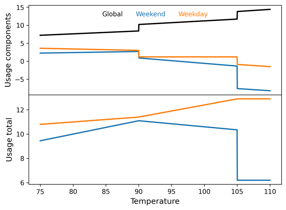
In this example, the building has decreased usage during the weekend and completely different behavior between weekdays and weekends in high temperature weather.
Solar Irradiance (Optional)🔗
It is unsurprising that buildings with solar PV generation respond to solar irradiance. Therefore, to model a building with solar PV production well requires a solar irradiance covariate as an input. The solar model expects a Global Horizontal Irradiance (GHI) time series to act as that covariate. GHI provides a direct proxy for solar generation, being approximately linearly proportional to PV production. The model assumes a linear response to GHI that is the same across all hours of the year.
It is currently up to the user to obtain their own GHI data. This can be done with free, but delayed, sources such as NREL or through a commercial service. The irradiance data should be location-specific either by weather station or directly over the meter location. Clearsky GHI should not be used as it neglects cloud cover which will impact PV production.
Solar irradiance is only required for the solar hourly model. If solar irradiance is not provided, the hourly model defaults to using the non-solar model.
Supplemental Data (R&D Only)🔗
The hourly model was specifically designed to be easily extended with supplemental data. These data could be pump or EV charging schedules. Any inputs will be treated with a linear response. Inputs can be either time series or catagorical, but cannot contain any missing values. The Correlation-based Imputation methodology is not used on supplemental data because it cannot be known if the imputation methodology makes sense for any arbitrary input.
Use of Supplemental Data is not approved by the working group for measurement.
This is meant to be a development feature to make it easier to improve the hourly model by testing proposed inputs.
Robust, Adaptive Outlier Downweighting🔗
While the majority of the time Sum of Squares Error (SSE) is the optimal metric to minimize to obtain the best model, there are instances where it is less effective at creating predictive models in data containing influential outliers. The hourly model handles these outliers by downweighting them using a robust, adaptive loss function and procedure on a per hour basis.
Model Fit🔗
Inputs into the model are provided through a dataframe to the appropriate data class. Internally, the model converts the inputs into a form appropriate for the underlying elastic net regression framework. When the model is fit, each site will receive its own unique model fit and coefficients.
Real Data Example🔗
It is rare to look at how the hourly model predicts for any given hour due to the high variance in hourly interval data, but let’s first look at the first 2 weeks in July for this solar, residential meter in its baseline period.
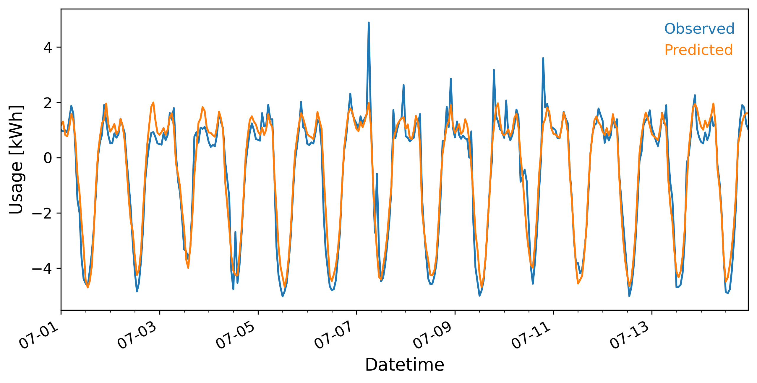
Here it looks like the model is performing fairly well, but this is only 672 hours out of a 8760 hour baseline year. Because of the large day-to-day variance, if we were to plot the entire year, it would be very difficult to glean any information from the smudge of a plot. Instead, let’s see what it looks like as a seasonal, hour-of-week loadshape.
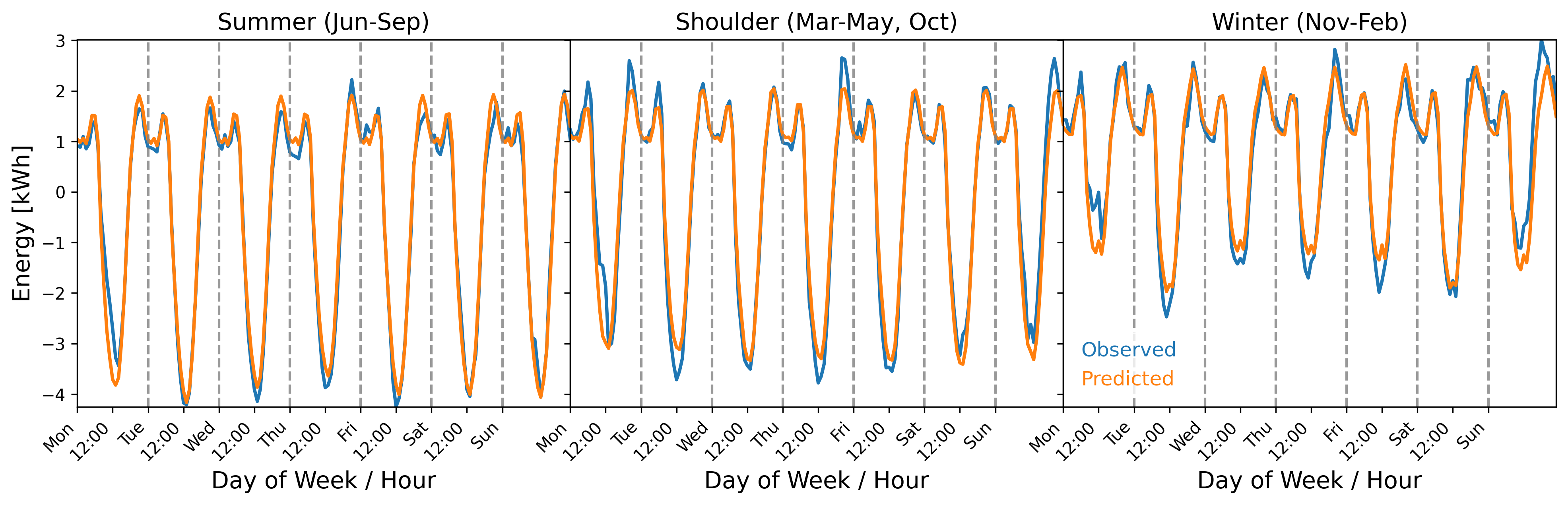
The seasonal, hour-of-week loadshape does confirm our prior assessment of how well the model is fitting the baseline data.