Methodology

The daily model is trained using daily energy usage intervals and predicts in daily intervals.

One of the key requirements of the daily model is to be able to disaggregate daily heating and cooling loads.

Model Theory

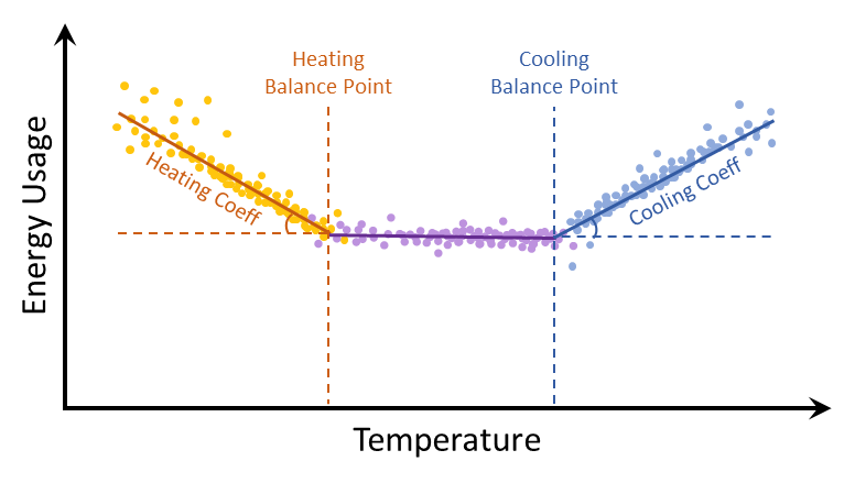
Model Shape and Balance Points

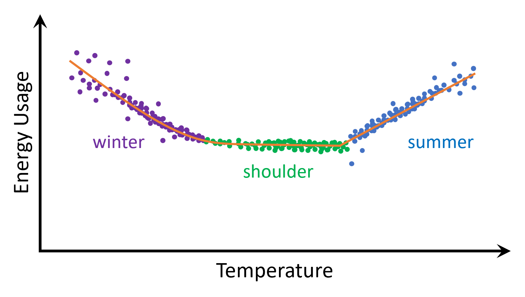
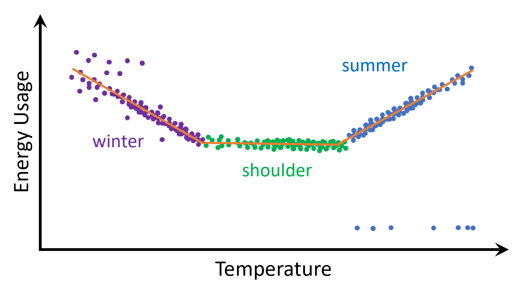
The daily model, at its core, utilizes a piecewise linear regression model that predicts energy usage relative to temperature. The model determines temperature balance points at which energy usage starts changing relative to temperature.

Nomenclature

• Balance Points: Outdoor temperature thresholds beyond which heating and cooling effects are observed.
• Heating and Cooling Coefficients: Rate of increase of energy use per change in temperature beyond the balance points.
• Temperature Independent Load: The regression intercept (height of the flat line in the diagram).

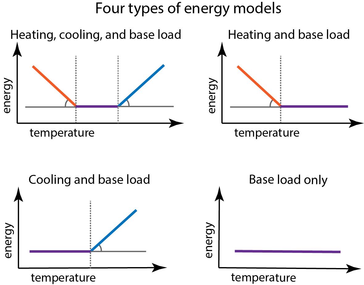
Model Archetypes

Based on the site behavior, there are four different model types that may be generated:

• Heating and Cooling Loads
• Heating Only Load
• Cooling Only Load
• Temperature Independent Load

Smooth Transitions

The daily model is designed to allow smooth transitions between model regimes. There are many reasons why a smooth transition might be favorable, but one example of this is inlet water temperature into a water heater. In this example, more energy will be required as the temperature decreases, which will be a smooth transition.

Robust, Adaptive Outlier Downweighting

While the majority of the time Sum of Squares Error (SSE) is the optimal metric to minimize to obtain the best model, there are instances where it is less effective at creating predictive models in data containing influential outliers. The daily model handles these outliers by downweighting them using a robust, adaptive loss function and procedure.

Model Fit

When the model is fit, each site will receive its own unique model fit and coefficients. The general model fitting process is as follows:

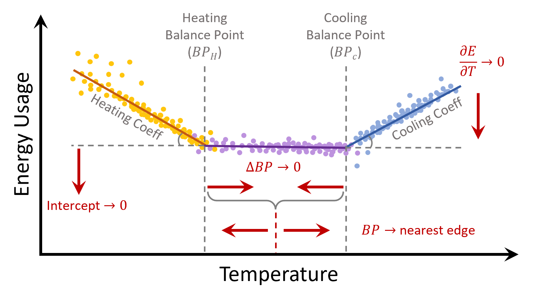
1. Balance points are estimated with a global optimization algorithm.
2. Sum of Squares Error (SSE) is minimized with Lasso inspired penalization.
3. The best model type is determined (ex. cooling load only model) using the penalized SSE.

The Lasso inspired penalization means that increased model complexity must be justified by decreased SSE and balanced against these general rules:

• Slopes are pushed to 0
• Intercept is pushed to 0
• Balance points are pushed together
• Balance points are pushed towards the nearest edge (most extreme temperature)
• Smoothing parameter is pushed to 0 (no smoothing)

Model Splits

The process described above is effective but may have shortcomings in real life data if energy usage changes fundamentally during different time periods.

For example, what if a site is more populated during a particular season (for example, a Summer House or Ski Lodge) or during weekdays (for example, offices and most homes). This may result in models that fail to accurately predict energy usage because they are trying to account for all time periods at once.

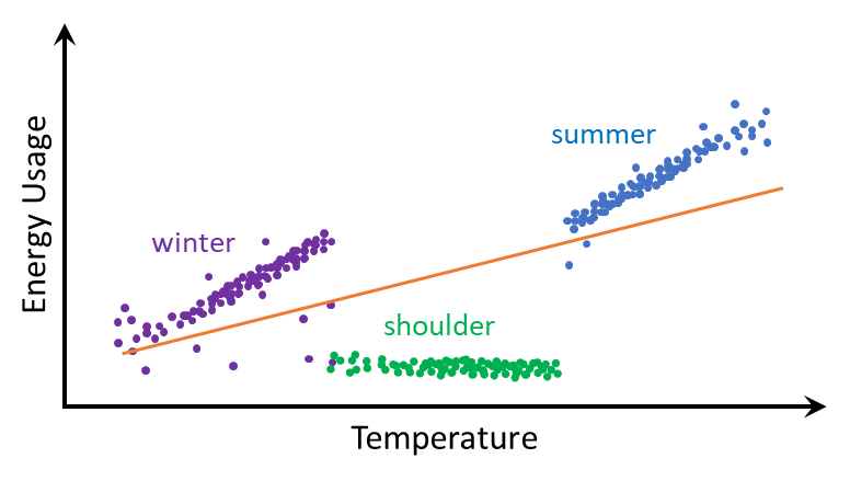
To combat this, the model will create “splits” that will store independent submodels for different seasons or weekday/weekend combinations, but only if necessary.

The general process is as follows:

1. Create submodels using all possible splits of season/weekday|weekend.
2. Calculate modified BIC (Bayesian Information Criterion) for each preliminary combination.
3. Select best combination with the smallest BICmod.

This provides a standardized process for splitting the model to better predict energy usage by certain time periods (if the benefit outweighs the additional model complexity).

---

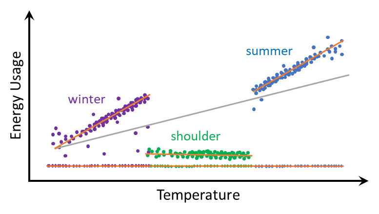
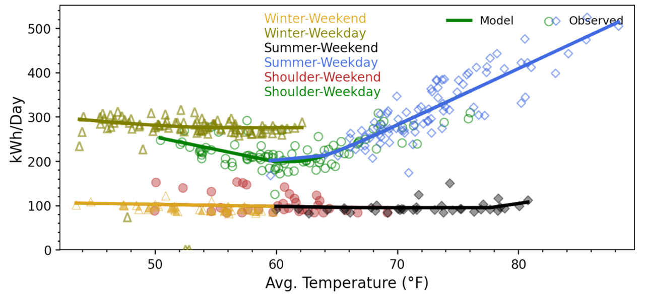
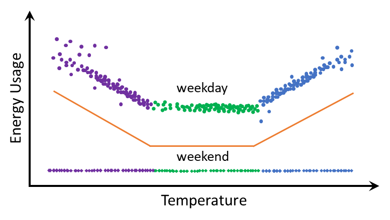
Real Data Example

The daily model is a deceptively complex model capable of handling some complex situations.

In this real example, we have three models:

1. Summer/shoulder weekday model: a smoothed model with heating, temperature independent, and cooling regions.
2. Winter weekday model: a model with heating and temperature independent regions that relies on adaptive downweighting (see the influential points at 0 kWh/day)
3. Weekend model: an all-season model with significant usage decrease compared to the weekday models.

For additional information and validation details, see References.