Example
In this example, we’ll walk through creating a Daily Model and predicting usage with it.
You can find a working example in the Example Code at the bottom of the page.
1) This example makes use of Matplotlib. Matplotlib is not a required dependency of OpenDSM.
2) If you run this example, it will download up to 150 MB of example data from the GitHub repo.
Imports🔗
import numpy as np
import matplotlib.pyplot as plt

import opendsm as odsm
from opendsm import eemeter as em
Loading data🔗
The essential inputs to OpenDSM library functions are the following:
- Meter baseline data named
observed - Meter reporting data
observed - Temperature data from a nearby weather station for both named
temperature - All data is expected to have a timezone-aware datetime index or column named
datetime
Users of the library are responsible for obtaining and formatting this data (to get weather data, see EEweather, which helps perform site to weather station matching and can pull and cache temperature data directly from public (US) data sources).
We utilize data classes to store meter data, perform transforms, and validate the data to ensure data compliance. The inputs into these data classes can either be pandas DataFrame if initializing the classes directly or Series if initializing the classes using .from_series.
The test data contained within the OpenDSM library is derived from NREL ComStock simulations.
If working with your own data instead of these samples, please refer directly to the excellent pandas documentation for instructions for loading data (e.g., pandas.read_csv).
Important notes about data🔗
- These models were developed and tested using temperature in units of °Fahrenheit. Please convert your temperatures accordingly
- It is expected that all data is trimmed to its appropriate time period (baseline and reporting) and does not contain extraneous datetimes
Let us begin by loading some example data. Here we use a built-in utility function to load some example data.
This function returns two dataframes of daily electricity data, one for the baseline period and one for the reporting period.
If we inspect these dataframes, we will notice that there are 100 meters for you to experiment with, indexed by meter id and datetime.
Returns
id      datetime                   temperature      observed
108618  2018-01-01 00:00:00-06:00    -2.384038  16635.193673
        2018-01-02 00:00:00-06:00     1.730000  15594.051162
        2018-01-03 00:00:00-06:00    13.087946  11928.025899
        2018-01-04 00:00:00-06:00     4.743269  14399.333812
        2018-01-05 00:00:00-06:00     4.130577  14315.101721
        ...                                ...           ...
120841  2018-12-27 00:00:00-06:00    52.010625   1153.749811
        2018-12-28 00:00:00-06:00    35.270000   1704.076968
        2018-12-29 00:00:00-06:00    29.630000   2151.225729
        2018-12-30 00:00:00-06:00    34.250000   1331.123954
        2018-12-31 00:00:00-06:00    43.311250   1723.397349
To simplify things, we will filter down to a single meter for the rest of the example. Let’s filter down to the 15th id.
n = 15

id = df_baseline.index.get_level_values(0).unique()[n]

df_baseline_n = df_baseline.loc[id]
df_reporting_n = df_reporting.loc[id]
If we inspect one of these dataframes, we will now notice that only a single meter is present with 365 days of data in each dataframe.
Returns
datetime                   temperature     observed
2018-01-01 00:00:00-06:00   -10.045000  9629.679232
2018-01-02 00:00:00-06:00    -4.712500  8868.878051
2018-01-03 00:00:00-06:00    11.352500  6109.322326
2018-01-04 00:00:00-06:00     0.972500  7557.067633
2018-01-05 00:00:00-06:00     3.147500  6650.189107
...                                ...          ...
2018-12-27 00:00:00-06:00    46.760000  2675.234259
2018-12-28 00:00:00-06:00    35.323125  3561.451294
2018-12-29 00:00:00-06:00    26.386250  3247.215055
2018-12-30 00:00:00-06:00    28.463750  3048.525124
2018-12-31 00:00:00-06:00    40.345250  3226.933132
Also notice the general structure of these dataframes for a single meter. We have three columns:
- A timezone-aware datetime index.
- A temperature column (float) in °Fahrenheit (be sure to convert any other units to °Fahrenheit first).
- Observed meter usage (float). The example here is electricity data in kWh, but it could also be gas data.
We can stop to plot this data to get a better understanding of the general behavior of this meter.
ax = df_baseline_n['observed'].plot(label='Observed Usage', color='blue')
df_baseline_n['temperature'].plot(ax=ax, secondary_y=True, label='Temperature (F)', color='orange')

ax.set_ylabel('Observed Usage (kWh)')
ax.right_ax.set_ylabel('Temperature (F)')

ax.legend(loc='upper left')
ax.right_ax.legend(loc='upper right')

plt.title('Observed Usage and Temperature in the Baseline Period')
plt.show()
Returns
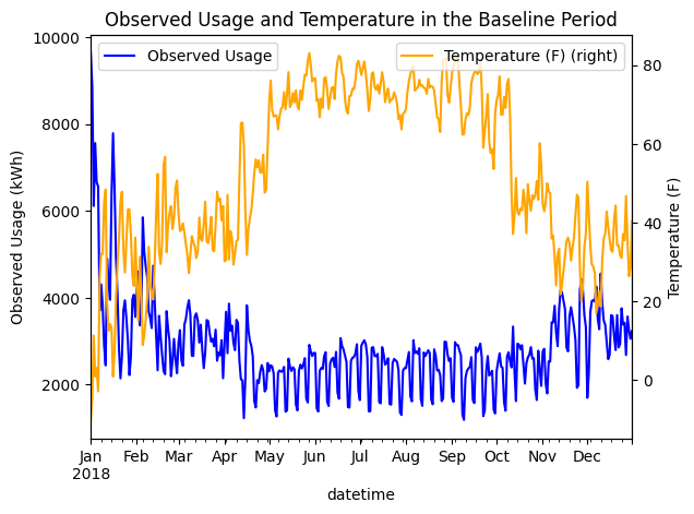
If we observe the data we can see a full year of data with observed usage peaking in the winter and lowering in the summer with warmer temperatures. It’s clear that this site is located in a colder climate and uses more electricity in the winter.
Loading Data into EEmeter Data Objects🔗
With our sample data loaded into dataframes, we can create our Baseline and Reporting Data objects. Note that only the baseline period is needed to fit a model, but we will use our reporting period data to predict against.
baseline_data = em.DailyBaselineData(df_baseline_n, is_electricity_data=True)
reporting_data = em.DailyReportingData(df_reporting_n, is_electricity_data=True)
These classes are critical to ensure standardized data loaded into the model. These classes also scan the data to check for data sufficiency and other criteria that might cause a model to be disqualified (unable to build a model of sufficient integrity).
As a note, you can also instantiate these data classes with two separate meter usage and temperature Series objects, both indexed by timezone-aware datetime.
Example
With data classes successfully instantiated, we can also check for any disqualifications or warnings before moving on to the model fitting step.
print(f"Disqualifications: {baseline_data.disqualification}")
print(f"Warnings:          {baseline_data.warnings}")
Returns
From this, we can see that no disqualifications are present but there are some warnings to be aware of as we proceed. Neither of these warnings will necessarily stop us from creating a model.
Before we move on, also notice that you can access the underlying dataframe in each object like follows to see exactly what will be loaded into the model.
Returns
datetime                   season  weekday_weekend  temperature  observed
2018-01-01 00:00:00-06:00  winter  weekday             -10.0450    9629.7
2018-01-02 00:00:00-06:00  winter  weekday              -4.7125    8868.9
2018-01-03 00:00:00-06:00  winter  weekday              11.3525    6109.3
2018-01-04 00:00:00-06:00  winter  weekday               0.9725    7557.1
2018-01-05 00:00:00-06:00  winter  weekday               3.1475    6650.2
Creating the Model🔗
The daily model follows the general process of:
- Initialize
- Fit
- Predict
We can do this easily as follows:
Before we move to predicting against a dataframe, we can actually use the built in plot function (requiring Matplotlib) to plot the performance of the model against the provided data.
Returns
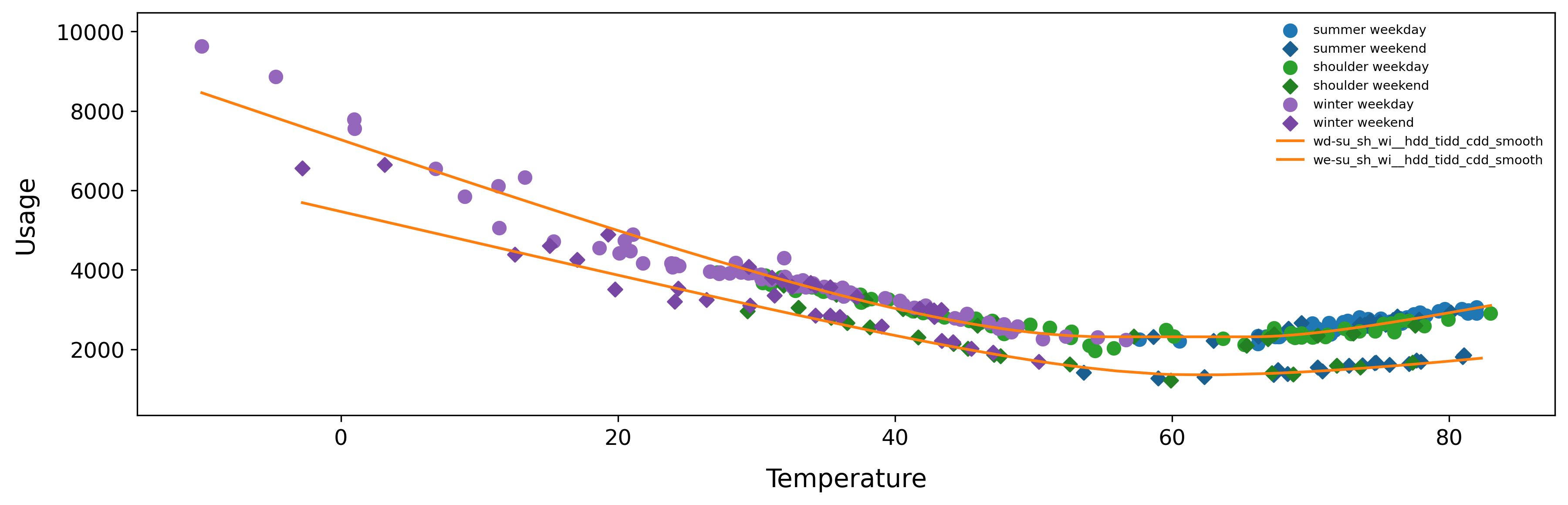
From this graph we can also observe model splits and model types as described in Model Splits. We can observe the following models:
- Summer/Shoulder/Winter - Weekday
- Summer/Shoulder/Winter - Weekend
This illustrates that the weekends are different enough to warrant their own model compared to the weekdays. Each meter is treated separately and will be given its own unique splits if justified by the data. All of this complexity is handled under the hood, and the model will utilize the correct model when predicting usage automatically.
We can also use this function to plot the model prediction against the reporting period as follows:
Returns
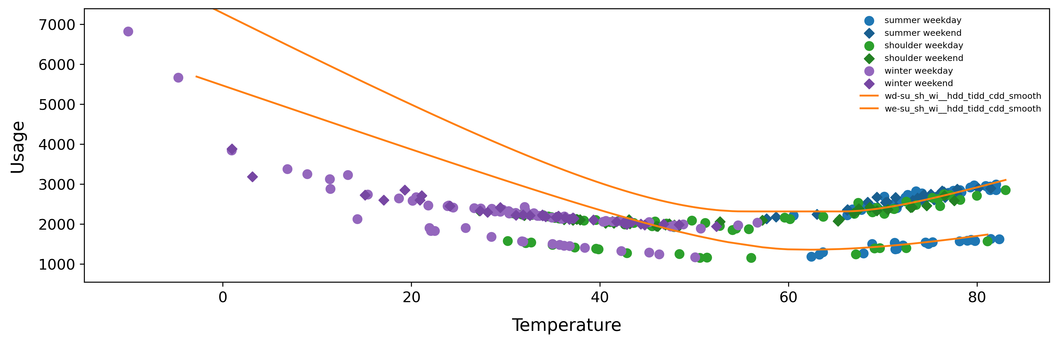
In this plot we can see that the site is using significantly less energy in colder temperatures compared to the model / baseline period. Perhaps this site installed an efficiency intervention that saves energy in colder temperatures?
Predicting with the Model and Calculating Savings🔗
With our fit model, we can now predict across a given reporting period as follows:
Returns
datetime season day_of_week weekday_weekend temperature observed predicted predicted_unc heating_load cooling_load model_split model_type
2019-01-01 00:00:00-06:00 winter 2 weekday -10.0450 6821.633670 8458.769369 403.385708 6145.508305 0.0 wd-su_sh_wi hdd_tidd_cdd_smooth
2019-01-02 00:00:00-06:00 winter 3 weekday -4.7125 5668.980225 7829.167990 403.385708 5515.906926 0.0 wd-su_sh_wi hdd_tidd_cdd_smooth
2019-01-03 00:00:00-06:00 winter 4 weekday 11.3525 3122.794390 5960.086410 403.385708 3646.825346 0.0 wd-su_sh_wi hdd_tidd_cdd_smooth
2019-01-04 00:00:00-06:00 winter 5 weekday 0.9725 3880.896300 7161.729548 403.385708 4848.468484 0.0 wd-su_sh_wi hdd_tidd_cdd_smooth
2019-01-05 00:00:00-06:00 winter 6 weekend 3.1475 3182.209058 5213.370264 285.516312 3858.054437 0.0 we-su_sh_wi hdd_tidd_cdd_smooth
We can also plot the observed usage vs. the predicted usage.
ax = df_results['observed'].plot(label='Observed Usage', color='blue')
df_results['predicted'].plot(ax=ax, label='Predicted Usage', color='orange')
ax.set_ylabel('Observed Usage (kWh)')
ax.legend(loc='upper left')
plt.title('Observed Usage and Temperature in the Baseline Period')
plt.show()
Returns
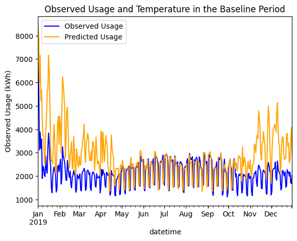
From here, we can easily calculate savings by subtracting observed usage from predicted usage.
df_results['savings'] = df_results['predicted'] - df_results['observed']
print(f"Predicted Usage (kWh): {round(df_results['predicted'].sum(), 2)}")
print(f"Observed Usage (kWh): {round(df_results['observed'].sum(), 2)}")
print(f"Savings (kWh): {round(df_results['savings'].sum(), 2)}")
Model Serialization🔗
After creating a model, we can also serialize it for storage and read it back in later.
Returns
{"submodels": {"wd-su_sh_wi": {"coefficients": {"model_type": "hdd_tidd_cdd_smooth", "intercept": 2313.2610638676033, "hdd_bp": 41.27040090608855, "hdd_beta": 119.44918113103105, "hdd_k": 0.4726274184833831, "cdd_bp": 70.96439586012724, "cdd_beta": 64.46865583811494, "cdd_k": 0.17605359829111333}, "temperature_constraints": {"T_min": -10.045, "T_max": 83.00500000000001, "T_min_seg": 8.94425, "T_max_seg": 81.38}, "f_unc": 403.3857082521867}, "we-su_sh_wi": {"coefficients": {"model_type": "hdd_tidd_cdd_smooth", "intercept": 1355.3158273422803, "hdd_bp": 50.8894292209749, "hdd_beta": 80.73766873918538, "hdd_k": 0.4482831249857758, "cdd_bp": 74.53352300727671, "cdd_beta": 41.0269706642773, "cdd_k": 0.5237054341526147}, "temperature_constraints": {"T_min": -2.7850000000000015, "T_max": 82.34, "T_min_seg": 22.4675, "T_max_seg": 79.7525}, "f_unc": 285.5163122905078}}, "info": {"metrics": {"num_model_params": 14, "wrmse": 218.75309123080092, "n": 365, "n_prime": 125.66853004788871, "ddof": 351, "ddof_autocorr": 111.66853004788871, "observed": {"sum": 1038753.15993621, "mean": 2845.899068318384, "variance": 1143760.7395673955, "std": 1069.4675028103452, "cvstd": 0.37579249198120157, "sum_squared": 3373659320.017336, "median": 2697.2358494980817, "MAD_scaled": 602.7295755197579, "iqr": 953.5552891155535, "skew": 2.221492866364899, "kurtosis": 9.332585130726638}, "predicted": {"sum": 1038740.3421026455, "mean": 2845.863950966152, "variance": 1074489.9131218037, "std": 1036.5760527437453, "cvstd": 0.3642394965479058, "sum_squared": 3348302512.293626, "median": 2627.7907614770256, "MAD_scaled": 464.5595323515464, "iqr": 914.7262255954338, "skew": 1.616695269464077, "kurtosis": 4.280790657230931}, "residuals": {"sum": 12.81783356446158, "mean": 0.03511735223140159, "variance": 47852.91368980268, "std": 218.7530884120329, "cvstd": 6229.202218054072, "sum_squared": 17466313.946906358, "median": 11.83559927083752, "MAD_scaled": 113.71324840144126, "iqr": 154.18635619428915, "skew": 1.3547762272723773, "kurtosis": 15.583344758089789}, "max_error": 1593.5483136788926, "mae": 126.71422886475526, "nmae": 0.044525201288895165, "pnmae": 0.13288608464673915, "medae": 76.1375240548914, "mbe": 0.03511735223140159, "nmbe": 1.233963376366405e-05, "pnmbe": 3.682780918133632e-05, "sse": 17466313.946906358, "mse": 47852.914923031116, "rmse": 218.75309123080092, "rmse_autocorr": 372.8098372555297, "rmse_adj": 223.07303332387448, "rmse_autocorr_adj": 395.4897491902344, "cvrmse": 0.07686607500105763, "cvrmse_autocorr": 0.1309989666906282, "cvrmse_adj": 0.07838402837514766, "cvrmse_autocorr_adj": 0.1389682977843363, "pnrmse": 0.22940787359451376, "pnrmse_autocorr": 0.39096824432836, "pnrmse_adj": 0.23393822662425828, "pnrmse_autocorr_adj": 0.41475282419864834, "r_squared": 0.9582550959309059, "r_squared_adj": 0.9565852997681421, "mape": 0.04085618887177056, "smape": 0.04056430298847941, "wape": 0.04452520128889517, "swape": 0.04452547600292869, "maape": 0.04074758380763742, "nse": 0.9581617787115769, "nnse": 0.9598419212949566, "kge": 0.9627155493651588, "a10": 0.9178082191780822, "a20": 0.9972602739726028, "a30": 1.0, "wi": 0.9890978278885424, "index_of_agreement": 0.9106627590653706, "pearson_r": 0.9789050494970932, "pi": 0.968232858166701, "pi_rating": "excellent", "explained_variance_score": 0.9581617797897993}, "baseline_timezone": "America/Chicago", "disqualification": [], "warnings": [{"qualified_name": "eemeter.sufficiency_criteria.extreme_values_detected", "description": "Extreme values (outside 3x IQR) must be flagged for manual review.", "data": {"n_extreme_values": 8, "median": 2697.2358494980817, "upper_quantile": 3269.296428540127, "lower_quantile": 2315.7411394245737, "lower_bound": -544.9247279220867, "upper_bound": 6129.962295886788, "min_value": 1181.0132889040156, "max_value": 9629.679232340746}}]}, "settings": {"developer_mode": false, "algorithm_choice": "nlopt_sbplx", "initial_guess_algorithm_choice": "nlopt_direct", "full_model": "hdd_tidd_cdd", "allow_smooth_model": true, "alpha_minimum": -100, "alpha_selection": 2, "alpha_final_type": "last", "alpha_final": "adaptive", "final_bounds_scalar": 1, "regularization_alpha": 0.001, "regularization_percent_lasso": 1, "segment_minimum_count": 6, "maximum_slope_oom_scalar": 2, "initial_step_percentage": 0.1, "split_selection": {"criteria": "bic", "penalty_multiplier": 0.24, "penalty_power": 2.061, "allow_separate_summer": true, "allow_separate_shoulder": true, "allow_separate_winter": true, "allow_separate_weekday_weekend": true, "reduce_splits_by_gaussian": true, "reduce_splits_num_std": [1.4, 0.89]}, "season": {"january": "winter", "february": "winter", "march": "shoulder", "april": "shoulder", "may": "shoulder", "june": "summer", "july": "summer", "august": "summer", "september": "summer", "october": "shoulder", "november": "winter", "december": "winter", "options": ["summer", "shoulder", "winter"]}, "weekday_weekend": {"monday": "weekday", "tuesday": "weekday", "wednesday": "weekday", "thursday": "weekday", "friday": "weekday", "saturday": "weekend", "sunday": "weekend", "options": ["weekday", "weekend"]}, "uncertainty_alpha": 0.1, "cvrmse_threshold": 1, "pnrmse_threshold": 1.6}}
Afterwards, we can instantiate the model as follows:
Automatic Sufficiency Checking🔗
Two of the core features of the OpenDSM Data and Model classes are automatic data sufficiency and model sufficiency checking. This ensures that only acceptable data and models are allowed to be used for making measurements. Let’s show an example of how this works by introducing too many NaN values into the observed data of the prior example.
# set rows 1:38 of observed to nan
df_baseline_n_dq = df_baseline_n.copy()
df_baseline_n_dq.loc[df_baseline_n_dq.index[1:38], "observed"] = np.nan
baseline_data_DQ = em.DailyBaselineData(df_baseline_n_dq, is_electricity_data=True)
print(f"Disqualifications: {baseline_data_DQ.disqualification}")
Returns
If this data were to try to be fit on it would return an error by default.
try:
daily_model = em.DailyModel().fit(baseline_data_DQ)
except Exception as e:
print(f"Exception: {e}")
In some circumstances it may still be possible to fit a model on disqualified data for investigative purposes. This can be done by setting the ignore_disqualification flag to True.
Please remember that enabling ignore_disqualification or making any changes to the model configuration fundamentally alters the model and such models are not approved for measurement purposes.
Example Code🔗
import numpy as np
import matplotlib.pyplot as plt
import opendsm as odsm
from opendsm import eemeter as em
df_baseline, df_reporting = odsm.test_data.load_test_data("daily_treatment_data")
n = 15
id = df_baseline.index.get_level_values(0).unique()[n]
df_baseline_n = df_baseline.loc[id]
df_reporting_n = df_reporting.loc[id]
baseline_data = em.DailyBaselineData(df_baseline_n, is_electricity_data=True)
reporting_data = em.DailyReportingData(df_reporting_n, is_electricity_data=True)
print(f"Disqualifications: {baseline_data.disqualification}")
print(f"Warnings: {baseline_data.warnings}")
daily_model = em.DailyModel()
daily_model.fit(baseline_data)
# Save model to json
saved_model = daily_model.to_json()
loaded_model = em.DailyModel.from_json(saved_model)
# Model results
daily_model.plot(baseline_data)
daily_model.plot(reporting_data)
df_results = daily_model.predict(reporting_data)
df_results['savings'] = df_results['predicted'] - df_results['observed']
print(f"Predicted Usage (kWh):  {round(df_results['predicted'].sum(), 2)}")
print(f"Observed Usage (kWh):   {round(df_results['observed'].sum(), 2)}")
print(f"Savings (kWh):          {round(df_results['savings'].sum(), 2)}")